Xf-Rovim. A Field Robot to Detect Olive Trees Infected by Xylella Fastidiosa Using Proximal Sensing

Abstract

The use of remote sensing to map the distribution of plant diseases has evolved considerably over the last three decades and can be performed at different scales, depending on the area to be monitored, as well as the spatial and spectral resolution required. This work describes the development of a small low-cost field robot (Remotely Operated Vehicle for Infection Monitoring in orchards, XF-ROVIM), which is intended to be a flexible solution for early detection of Xylella fastidiosa (X. fastidiosa) in olive groves at plant to leaf level. The robot is remotely driven and fitted with different sensing equipment to capture thermal, spectral and structural information about the plants. Taking into account the height of the olive trees inspected, the design includes a platform that can raise the cameras to adapt the height of the sensors to a maximum of 200 cm. The robot was tested in an olive grove (4 ha) potentially infected by X. fastidiosa in the region of Apulia, southern Italy. The tests were focused on investigating the reliability of the mechanical and electronic solutions developed as well as the capability of the sensors to obtain accurate data. The four sides of all trees in the crop were inspected by travelling along the rows in both directions, showing that it could be easily adaptable to other crops. XF-ROVIM was capable of inspecting the whole field continuously, capturing geolocated spectral information and the structure of the trees for later comparison with the in situ observations.

1. Introduction

Xylella fastidiosa (X. fastidiosa) was first detected in Italy (Apulia region, southern Italy) in 2013 [1], and it has since spread rapidly throughout the region causing severe damage to olive crops. Its detection throughout Corsica (France) and in south-eastern France, along with the more recent outbreaks in Mallorca (2016), Alicante (2017) and Madrid (2018), in Spain [2], have greatly increased the awareness of the threat that this pathogen poses to European agriculture and the environment [3]. As a consequence of the X. fastidiosa outbreak in Italy affecting mostly olive trees, almost the entire province of Lecce (Apulia Region) has been declared an area under containment [4]. The project XF-ACTORS (EU H2020 727987) tackles these problems from a multidisciplinary research approach. The solutions proposed include the setting up of proximal and remote-sensing tools for early diagnostic and surveillance programmes. However, the representativeness of diagnostics relies heavily on proper sampling design, which should include both the field and the individual plant level with fine resolution, but also large spatial coverage that can only be achieved through extensive testing.

Spectral remote detection collects information by measuring the radiance emitted, reflected and transmitted from the vegetation. The sensors used to obtain this information, such as red, green and blue (RGB) cameras, spectral imaging systems, point spectrometers or thermographic cameras, measure the electromagnetic energy reflected or emitted by the vegetation in different spectral ranges or at particular wavelengths [5]. This information is affected by several structural and biochemical components of the plants, such as leaf area, porosity, chlorophyll and water content or nitrogen concentration, which can change and thus result in stresses that are potentially detectable by these spectral devices [6]. In addition, fluorescence emission and canopy temperature can be quantified from remote sensing images, which are directly related to plant photosynthesis and transpiration rates and are used for the early detection of stresses that can be caused by diseases or invasion by pests [7]. For these reasons, both healthy and diseased plants have particular spectral signatures, which allow detection of the physiological and biochemical effects of the early stages of the infection, for example, by the use of vegetative indices [8]. In addition, some information can be obtained from the study of the 3D structure of plants [9], which can be affected as a result of serious diseases. This information can be collected using detection devices capable of obtaining the structure of the plants by measuring the distance between the device and the plant and creating its point cloud, such as stereo cameras, time-of-flight cameras or laser scanners. One of the most widely used sensors in the field for this purpose is a light detection and ranging (LiDAR) sensor, which is a device that can measure the distance to the nearest object by emitting a laser beam in a given direction; the time elapsed between the emission and reception of the signal is then used to calculate the distance to the target. Therefore, by crossing the entire plant with the sensor, geometric parameters such as height, width, volume and other structural parameters of the canopy can be estimated [10]. Moreover, the laser pulses emitted by the LiDAR sensor can penetrate through the canopy and, thus, the effects of shading or saturation are reduced [11,12].

The use of remote sensing to map the distribution of plant diseases has evolved considerably over the last three decades and can be performed at different scales, depending on the area to be monitored as well as the spatial and spectral resolution required [13]. Apart from satellites, which are necessary when very large regions need to be covered, manned aircraft remain the only alternative to obtain maps at larger scales with optimum spatial and spectral resolution for the early detection of disease outbreaks [14]. In [15], the authors demonstrated that the use of airborne imaging spectroscopy and thermography allows the detection of symptomatic olive trees infected by X. fastidiosa as well as the prediction of the infection before the symptoms are visible, with an accuracy of above 80%. They surveyed more than 7000 trees by means of a manned aircraft, using hyperspectral and thermal sensors to capture information about the physiological alteration of the trees caused by X. fastidiosa. The information was confirmed by visual observations and molecular analyses of selected trees using quantitative polymerase chain reaction. Their findings indicated that it is possible to perform accurate detections of the infection by X. fastidiosa at landscape level by using remote sensing equipment, in particular, hyperspectral imaging and thermography.

At the plant level, the spectral information has to be gathered at high spatio-temporal resolution. Sensors for this purpose can be mounted on unmanned aerial vehicle (UAV) platforms to obtain low-cost imagery at spatial resolutions from 1 to 100 cm [16]. However, when higher spatial resolutions are required (from the plant to a leaf level) hand-held devices or sensors mounted on ground vehicles are a good solution [17]. In [18], the authors tested different sensing technologies, including an ultrasonic sensor, a LiDAR sensor, a Kinect camera and an imaging array of four high-resolution cameras mounted on a ground vehicle platform to measure the plant height in the field. They compared the performance of these sensors with the images captured by a camera mounted on a UAV, concluding that data obtained from the ground achieved higher correlations than aerial images. In [19], a ground vehicle equipped with a multispectral imaging system was also employed to obtain vegetative indices that were used to characterise the vine foliage of several varieties of grapevine. In [20], the authors developed the Shrimp robotic ground-vehicle, which was used as an information collection system for almond orchard mapping and yield estimation. The sensing system continuously recorded data while the vehicle drove through the orchard. The equipment included a LiDAR, a colour camera, a gamma radiometer to record passive soil gamma emissions and an electromagnetic induction instrument to measure apparent soil electrical conductivity. Although unmanned vehicles have already been studied in agriculture to collect extensive information about the crop, when more detailed data need to be collected in complex environments, remotely driven vehicles equipped with sensing equipment are a realistic solution [21].

The aim of this work is to develop a flexible robotic-based approach with proximal sensing tools specifically developed to detect X. fastidiosa and to implement and test it in the field under real conditions. Therefore, a small ground robotic platform (X. fastidiosa—Remotely Operated Vehicle for Infection Monitoring, XF-ROVIM) was built for the early detection of X. fastidiosa, primarily in olive trees, but it is also adaptable to other crops.

2. Materials and Methods

2.1. Robotic Platform

Sensing technologies based on optical measurements that can be installed on all-terrain human-operated vehicles are already available for crop monitoring. However, some of the vehicles currently used for agricultural tasks are too large or they are dedicated to a single or a small group of crops. Autonomous vehicles are a good solution, but they need advanced navigation algorithms to deal with a complex and highly variable environment [22]. Hence, they often need to be programmed with precision to be able to work in the particular environment for which they are designed. When the vehicle with the sensing equipment has to work with different crops and under different terrain and environmental conditions, remote driving is an adequate option, especially if the availability of any regular vehicle in which to install the sensing equipment is not guaranteed for the test fields. Hence, the systems need to be small and the integration of the sensing equipment also needs to be improved to be able to create more usable and flexible solutions [23]. As X. fastidiosa can infect more than 560 host species [24], XF-ROVIM has been designed and built as a flexible platform that can work on different crops because of its small size, capability to be driven remotely and adaptability to crops with very different heights. One required restriction is a relatively small size so that it can be easily transported in a van, and hence its maximum size is 100 × 60 cm. Two accessible and easy-to-replace gel batteries power two direct current (DC) motors. A platform containing the cameras can be elevated up to 200 cm for better measurement of the highest trees, which is of special importance as the trees in the testing region are relatively tall (up to 6 m) and, in the early stages, the infection prevails in the upper part of the canopy [1].

To build the traction control board, two DC motor control drivers were used (H-Bridge), which allow the operator to control the speed and torque of the motors as well as their direction of rotation. The use of a driver for each wheel allows manoeuvres to be performed with greater precision, since one wheel can be braked in order to make turns or to run each wheel in opposite directions, thus reducing the angle of rotation. A rotary encoder was placed on one wheel, allowing accurate measurement of both speed and distance advanced. Based on the information from the encoder, which is processed by the controller, a trigger is sent to the equipment to obtain data synchronised with the forward movement. The board includes an 868 MHz radiofrequency module to communicate bi-directionally with a wireless controller. All the electronics on this board are managed by a 16-bit microcontroller (PIC24EP, Microchip Technology Inc., Chandler, AZ, USA). The range of the wireless connection is between 500 and 1000 m, depending of the crop structure and characteristics, which is in any case enough for this application.

The wireless control was designed to include a joystick that allows the robot to be steered, while a sliding potentiometer allows the speed to be adjusted (when the automatic mode is selected) in order to obtain greater precision. A selector allows the operator to choose between manual and automatic modes. When the automatic mode is selected, a proportional–integral–derivative (PID) controller continuously compares the speed set by the user with the speed read by the encoder and applies the necessary power to the motors in a closed loop process. In addition, another selector makes it possible to pre-set the advance distance at which the sensing equipment is to be triggered. All these elements are connected to an especially designed board, which includes another radiofrequency module. Apart from the sensing equipment, the cost of the robot itself is less than €5000.

2.2. Sensing Equipment

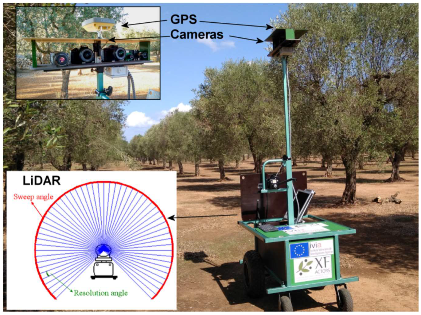
The sensors mounted on XF-ROVIM included two digital single-lens reflex (DSLR) cameras (EOS 600D, Canon Inc., Tokyo, Japan), one of them modified to obtain images showing the blue normalised difference vegetation index (BNDVI), a multispectral camera (CMS-V, Silios Technologies, Peynier, France) that can obtain simultaneous images at eight different wavelengths (558, 589, 623, 656, 699, 732, 769, and 801 nm), a low-cost hyperspectral system in the visible and near infrared (NIR) range between 400 nm and 1000 nm (spectrograph Imspector V10, Specim Spectral Imaging Ltd., Oulu, Finland + camera uEye 5220CP, iDS Imaging Development Systems GmbH, Obersulm, Germany) and a thermal camera (A320, FLIR Systems, Wilsonville, OR, USA). All cameras were configured to capture one image per metre, synchronised with the advance of the robot.

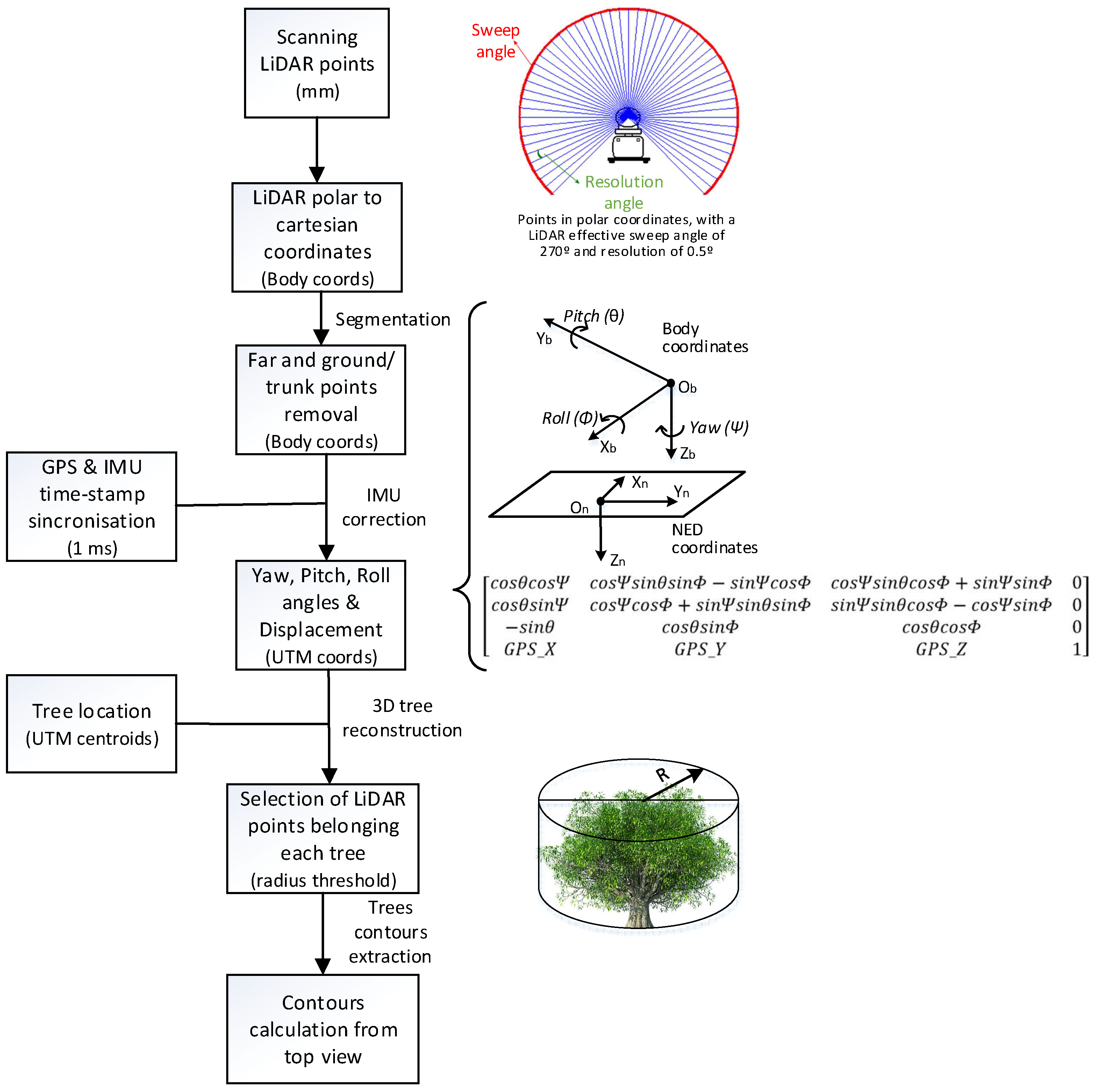
The equipment was completed with a LiDAR (LMS111, Sick AG, Reute, Germany) with an effective sweep angle of 270° and a resolution of 0.5°. All data were geolocated using a GPS with a horizontal positioning accuracy of 10 mm (Hiper SR, TOPCON Corp., Tokyo, Japan) and corrected by means of the data captured by an IMU based on a 9-axis absolute orientation sensor (BNO055, Adafruit learning system, USA). A general view of the robot and the sensing equipment is shown in Figure 1. The accuracy of the GPS was 25 cm, which was found to be sufficient to meet the requirements. The LiDAR, the GPS and the IMU were configured to operate in free range, with the highest resolution of each sensor. Accordingly, data from the three units were synchronised by means of the timestamp (with a resolution of 1 ms) provided in the data streams captured by each sensor. Apart from the sensing equipment, the setup is also equipped with an industrial computer, a folding screen and all the electronics required to capture the data.

2.3. Field Tests

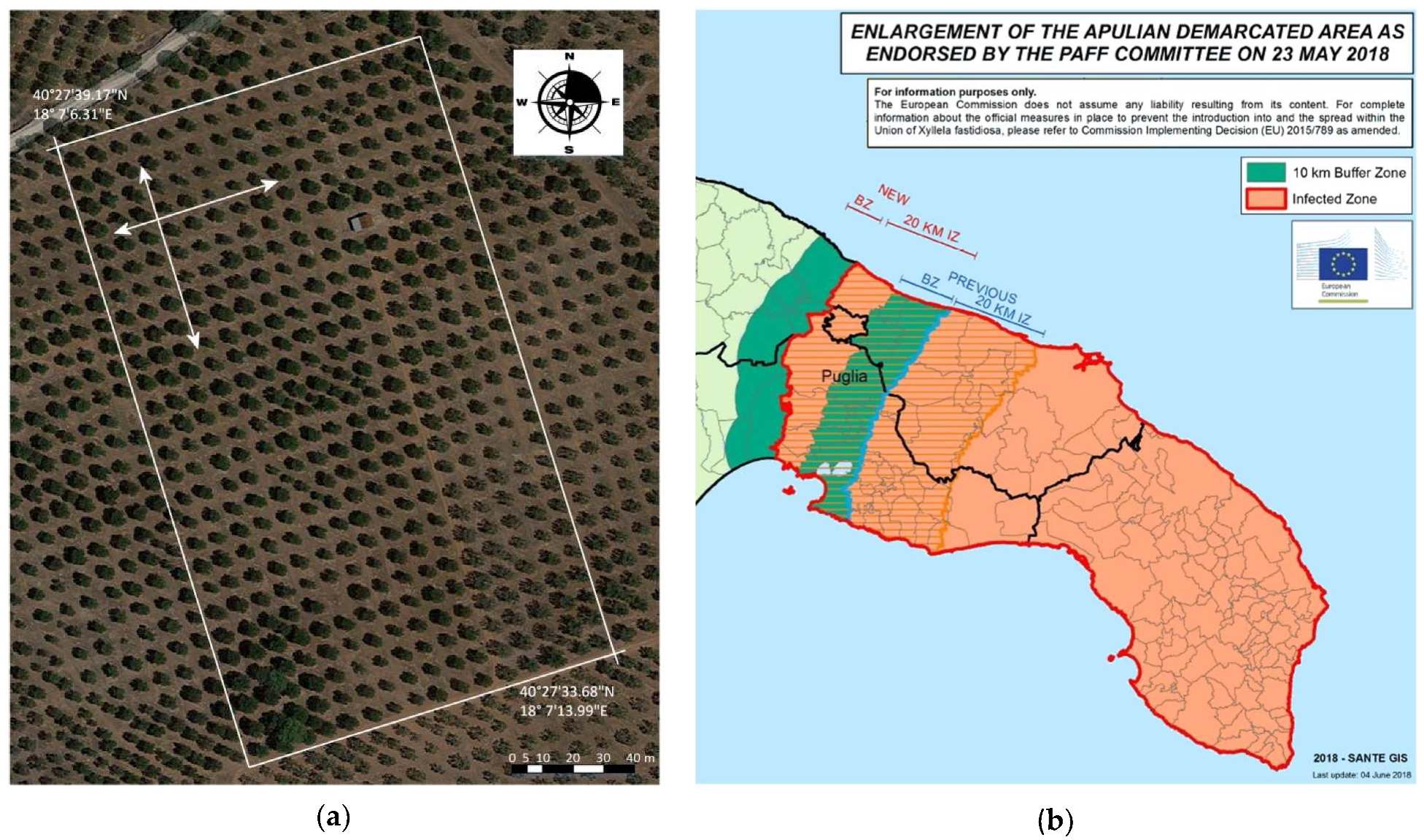
Field tests were carried out to test the performance of all the systems in a real environment, including the mechanics, the electronics, the geolocalisation and correction system, and how long the batteries lasted during the monitoring operation. Two experiments were carried out in the province of Lecce in September 2017 and June 2018, in an olive grove known as C20 (18.119561 latitude, 40.460148 longitude) with a surface area of 3 Ha (Figure 2a). This field has 430 olive trees cv. ‘Ogliarola’ and ‘Cellina di Nardò’. It is located in the contention area demarcated by the EU (Figure 2b). During both tests, XF-ROVIM was deployed in the field, advancing along each row at a speed of 1 m/s. The cameras are focused towards one side of the robot. Hence, as it advances along a row, only images of the trees located on one side of the row can be captured. When a row is finished, the robot must go back along the same row to obtain the images of the trees on the other side. After covering the entire field in one direction, the same inspection process was repeated in the perpendicular rows to image the north and south sides of each tree. The first surveys (September 2017) were used to fine-tune the electronics and to set up and programme all the sensors, collect preliminary data and improve autonomy and ease of handling. The more recent tests (June 2018) were carried out to collect data on the orchard status that will serve to detect the presence of the infection in the trees.

Each camera is different but all of them can be triggered externally. Thus, every time a trigger was generated, the cameras captured the images and stored them on the solid-state disk (SSD) of the computer for later analysis, except in the case of the DLSR cameras, which stored the images on their own secure digital (SD) card. When the inspection of a row was finished, a command on the remote control allowed all the images from the computer’s memory to be transferred to the SSD and to update the labels of the images with information about the next row to be inspected. The images acquired using the modified DLSR served to calculate the BNDVI index, while those captured by the multispectral camera at 800 nm and 670 nm were used to capture the NDVI index. Bearing in mind the specifications of each camera, the two indices were calculated as shown in Equations (1) and (2) respectively.

BNDVI = (850 nm − 480 nm)/(850 nm + 480 nm)

(1)

NDVI = (800 nm − 670 nm)/(800 nm + 670 nm)

(2)

Before, during and after the inspection, images of a standardised colour checker (ColorChecker SG Chart, X-Rite Inc., USA) and a white reference target (Spectralon 99%, Labsphere, Inc., North Sutton, NH, USA) were acquired for further image correction.

In addition, a visual inspection of each tree was carried out on the basis of the severity of its symptoms. Each of the four sides of the tree were measured on a rating scale of disease severity from 0 (no symptoms) to 4 (prevalence of dead branches) [15]. However, as the field is currently active, the farmer usually removes the branches in poor condition so that the visible symptoms do not always correspond to the actual degree of infection. This is a critical point to obtain reference data on early detection of asymptomatic infected trees, but does not affect the detection of the symptoms when present. Apart from measuring the visual symptoms, some trees were analysed using molecular biology techniques to detect the presence of the infection with greater accuracy.

2.4. Data Management

2.4.1. Tree Reconstruction from LiDAR Data

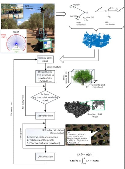
The data from the LiDAR, the GPS and the IMU sensors were stored in ASCII format, one file being recorded per row/column scanned. The LiDAR coordinates, originally in millimetres in a cylindrical coordinate system, were converted to metres in a Cartesian coordinate system and subsequently geolocated with the GPS reference using the WGS 84/UTM coordinates system in the 34T zone. These coordinates were later corrected by means of the IMU unit using the pitch, yaw and roll angles to minimise the impact of the roughness of the terrain experienced during the movement of the robot. The LiDAR sensor and the GPS and IMU units were synchronised by means of the timestamp in the data streams captured with a time resolution of one millisecond.

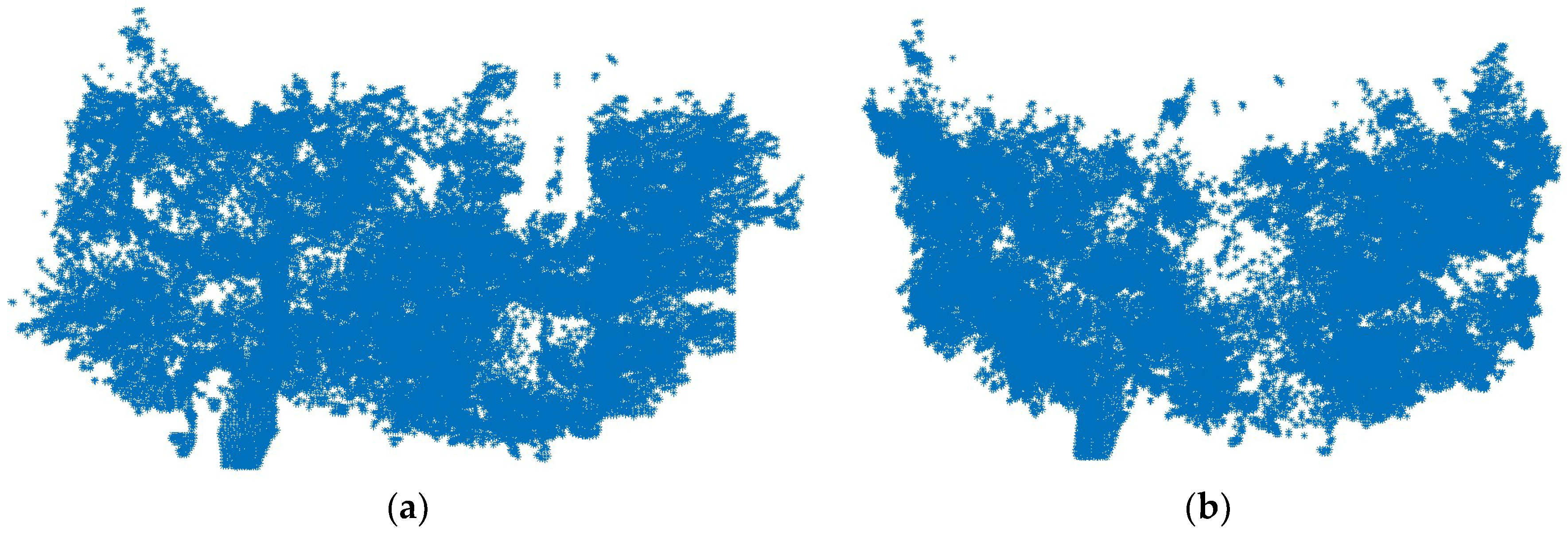
First, XF-ROVIM scanned the field with all the mounted sensors in the direction represented by arrows in Figure 2a and all the data gathered were stored in files. As an off-line process, the LiDAR points corresponding to each 270° sweep were converted from polar to Cartesian coordinates, fixing the origin of the coordinates at the position of the LiDAR (the so-called body coordinates) for that sweep. Then a filtering process was performed to remove the points that do not belong to the canopy, such as the ground, trunk and distant points. Different threshold values were applied to the scanned points according to the field configuration. First, a vertical threshold was determined, which corresponded to the height of the lowest leaves of the trees. All points with a lower height were discarded. Second, points scanned out of a given radius distance (considering a top view of the field) from the centre of the corresponding tree were also discarded. The body coordinates were later corrected using the Euler angles and the GPS location, which transformed them into Universal Transverse Mercator (UTM) coordinates (equivalent to NED—North–East–Down—system coordinates). The GPS location was used to geolocate the origin of the body coordinates and the Euler angles (Yaw Ψ, Pitch θ and Roll Φ) were used to orient the LiDAR points in space. Subsequently, the previously selected UTM centroids of each tree were used to reconstruct the trees. In this process, the LiDAR points close to each centroid and under a certain distance were chosen as belonging to a particular tree. This distance was set as half the distance between the rows of trees. Figure 3 shows one tree point cloud from the tree point cloud structure generated in this process. Lastly, the top views (horizontal projection of all the tree points in the NED plane) were used to extract the contour of the point cloud of each tree. The workflow of the entire process is shown in Figure 4, where the main steps of the algorithm developed are depicted.

All the software to analyse and process this information was developed in MATLAB (9.3 R2017b, The MathWorks Inc., USA).

2.4.2. Tree Leaf Indices Calculation

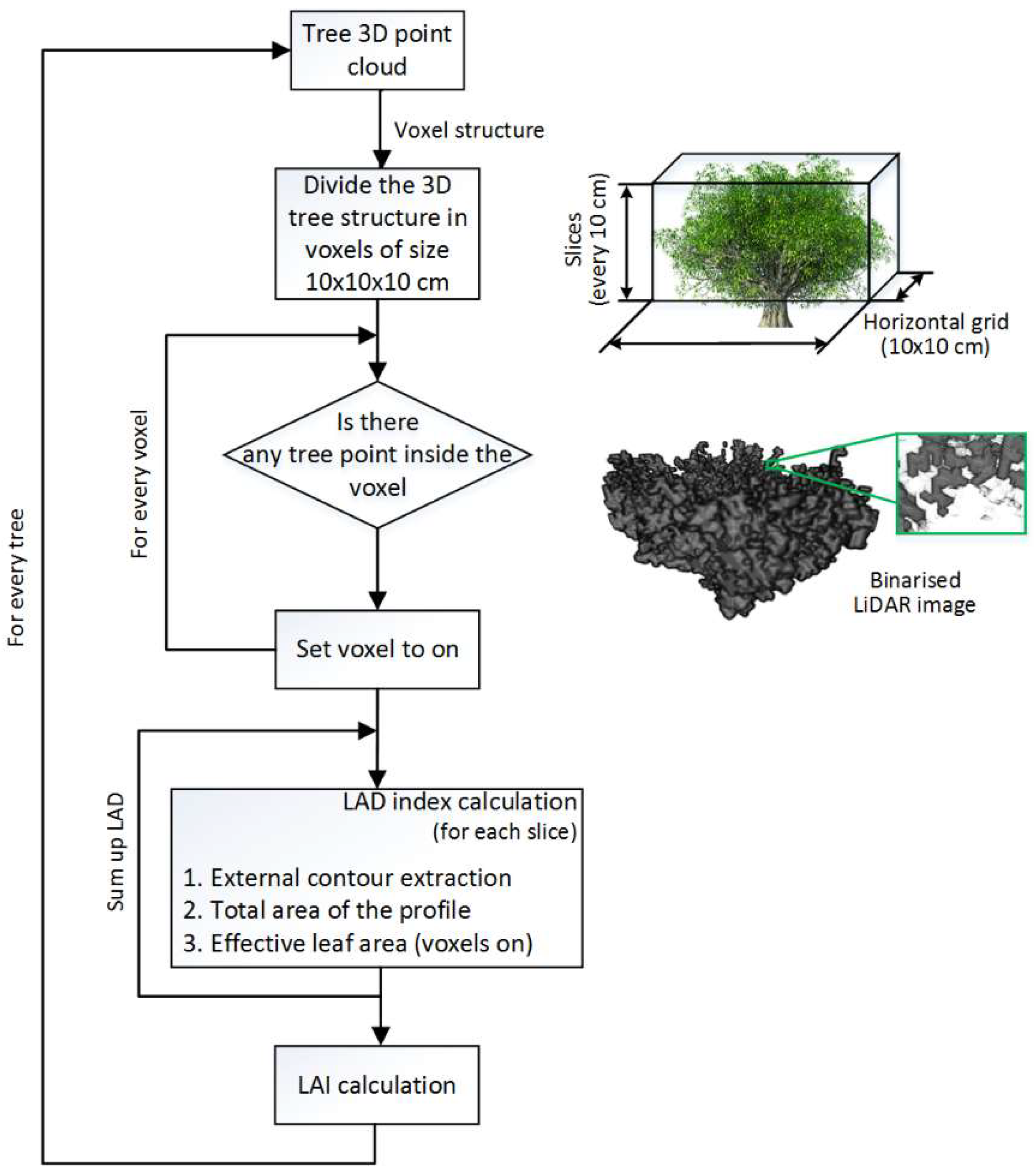
Once the LiDAR information was processed and the 3D tree structure was created, the tree leaf index (LAI) and the leaf area density (LAD) were calculated for each tree in particular, since they are some of the Main variables used to evaluate processes such as photosynthesis or evapotranspiration, which have a great influence on the reflectance of the canopy. The LAD is defined as the total one-sided leaf area of photosynthetic tissue per unit canopy volume, while the LAI is obtained by integrating the LAD over the height of the canopy [25]. There are different approaches to calculate these indices. This work adapted the method proposed by [26] based on the voxel-based canopy profile (VCP). Basically, as proposed by this method, the cloud of points of the tree was considered to be inside of a three-dimensional cube, which was divided into voxels (3D volume elements) with a resolution of 10 × 10 × 10 cm. Then, a voxel was set to “on” or “off” according to the presence or not of scanned points inside. In this way, each tree was represented by a 3D voxel-based structure integrated by the voxels set to “on” that belonged to the tree. Finally, the LAD and LAI calculations were performed following Equations (3) and (4). The LAD was calculated for each horizontal layer as the effective area density obtained as the voxel relation “on” in that layer and the total area of the tree’s contour in that layer. The LAI of the tree was calculated as the sum of the different LAD projected in the different layers to complete the height of the tree. The representation of the trees based on voxels allowed that 3D image techniques could be applied, thus facilitating all the necessary calculations. The overestimation problems were not considered, since the overlapping points in the LiDAR data were represented in the model as a single voxel. The flowchart describing this process is shown in Figure 5.

$$LAD=u\left(z\right)$$

(3)

In this equation, u = surface density coefficient of a layer in the tree foliage; z = specific height of the layer.

$$LAI\left(z\right)={{\displaystyle \int }}_{z=0}^{h}LAD\left(z\right)dz;$$

(4)

In m²m⁻² units, where h goes from 0 to tree height; LAD(z) = surface density coefficient.

The LAD indices were calculated using the different horizontal planes (XY planes) (Figure 6c), where the effective area calculated for each plane was the leaf area found inside the external contour of the profile in each plane.

3. Results and Discussion

3.1. Robotic Platform

XF-ROVIM worked properly during the tests in a field of relatively tall olive trees, as it was capable of continuously inspecting the whole field without interruptions while capturing valid data. During each survey, around 35,000 images (one every metre) were captured with all five cameras (colour, multispectral, hyperspectral, thermal and DLSR modified to capture BNDVI images). The remote driving unit was seen to be a flexible easy-to-use tool for moving the robot around the whole field. Some driving tests were conducted, which showed the possibility of surrounding each tree for a complete individualised inspection. Nevertheless, the decision was made to inspect entire rows. As the remote control could be programmed to maintain the speed and the direction once established, no intervention was needed during the inspection of the rows. The batteries lasted for more than six hours of continuous operation, and they could be changed for another set in less than 15 min.

The GPS ran in free mode at 25 Hz. As the robot was programmed to advance at a speed of 1 m/s, the location was captured approximately every 40 mm. For the images, the accuracy of the location was not a true problem, because only those images containing complete trees were selected (only one image per tree: those captured between consecutive trees were discarded). Then, every image could be properly associated with each tree. As the images of each tree were geolocated, all the trees in the field could also be geolocated with great accuracy. The association between an image and the GPS information was performed by timestamp. The millisecond in which each image was acquired was stored along with the image and associated with the closest timestamp of all GPS locations. The association between the LiDAR and the GPS was more critical, not because of the exact location but because the tree must be reconstructed with great precision. Equally, a timestamp with a precision of milliseconds was recorded along with the data. This timestamp allowed the data from the LiDAR to be associated with the closest GPS location with a high degree of accuracy. The system developed to raise the sensors to different heights allowed the equipment to adapt the measurements to the canopy of very tall trees. The information provided by the robot was used to obtain, measure and visualise the structure of the trees. In addition, the spectral images of all the trees were captured and used to obtain vegetative indices of each tree.

Other examples of scouting robots for crop surveillance can be found, but they have been developed to work only on specific crops and offer little information about the design, construction, functionalities and cost of the prototypes. Ladybird [27] is an autonomous multipurpose farm robot for surveillance, mapping, classification, growth monitoring, and pest detection for different vegetables using laser and hyperspectral scanning. Mantis [28] is a flexible general-purpose robotic data collection platform equipped with different sensors like RADAR, LiDAR and panospheric, stereovision and thermal cameras. The VineRobot (http://www.vinerobot.eu) and its continuation VineScout (http//www.vinescout.eu) are autonomous robots equipped with advanced sensors and artificial intelligence to monitor vineyards. VinBot [29] is another all-terrain mobile robot with advanced sensors for autonomous image acquisition and 3D data collection in vineyards used for yield estimation. GRAPE (http://www.grape-project.eu) is a ground robot also for vineyard scouting, plant detection and health monitoring, and even the manipulation of small objects. In general, brief descriptions of these solutions can be found but no information on their performance (of platforms and sensors) or tests have been published.

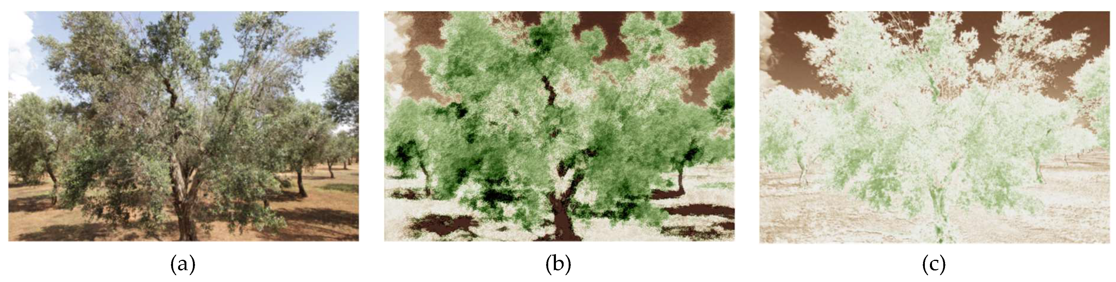
3.2. Data Collection

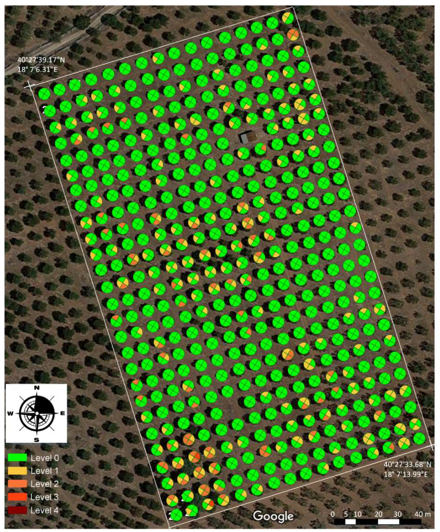
The external symptoms of disease observed by the visual inspection (levels 0 to 4) are shown in Figure 7. Most of the trees did not show any symptoms of the disease, probably due to the cleaning process carried out by the grower, but some others grouped in patches did show slight-to-moderate symptoms. Nonetheless, altogether 174 trees showed some symptom, mostly those on the west and north sides. The first results of the automated analysis of the NDVI and BNDVI indices of the trees from the captured images (Figure 8) achieved a coefficient of determination R² in relation to the observed symptoms lower than 0.45 in both cases, which indicates that these indices are not suitable in this problem, as already stated by Zarco-Tejada et al. in [15]. Moreover, as has been demonstrated in [15], other vegetative indices related to different pigments that involve wavelengths in the VIS/NIR range (400–1000 nm) are offering promising results in the detection of the infection by Xf in olive trees. These indices typically involve measurement at a wavelength associated with absorption of the pigment of interest, referenced by measurement at a wavelength used for background correction that is not affected by pigment absorbance, but scattering in the plant tissue. As these biochemical constituents can be altered by the stress caused by the infection [6], they are potentially detectable by the spectral devices incorporated in the robot.

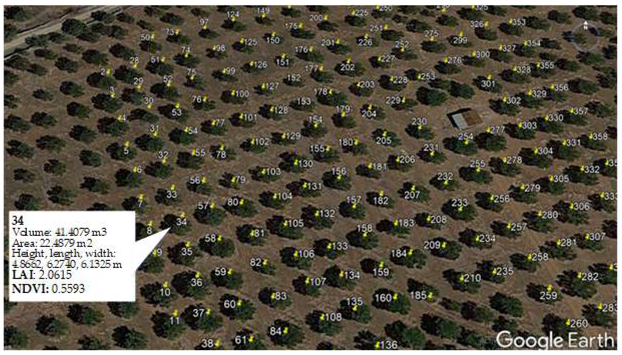
The LiDAR information allowed 3D reconstruction of the trees in a subsequent off-line process with a total execution time of 850 s for the entire field. The original polar points of the LiDAR were converted to UTM Cartesian coordinates and the points corresponding to ground or trunk were removed using different threshold values. The trees were later reconstructed from the points that were close to each tree centroid with a distance lower than a specific radius value, established as half the distance between two consecutive trees. The 3D structure of the tree was used to calculate dimensions such as height, length, width, top projected area and volume. In addition, the LAI (cumulative LAD) was calculated, thus providing important information about each individual tree that can later be compared to future scans to determine the changes in the evolution of the disease. The study of the temporal evolution can provide key information for early diagnostic and surveillance applications using proximal or remote-sensing tools. To facilitate the graphical visualisation of this information and the interaction with the user, key tree features were associated with numbered pushpins in the Google Earth application using KML language with MATLAB. Thus, when a user browses the field on Google Earth, key information about the tree pops up automatically on clicking on the tree pushpin. Figure 9 shows the top view of the orchard that was studied ready to obtain the information about any tree. An example of the information corresponding to tree 34 is detailed, showing the extracted features, including the LAI and NDVI indices. However, as in the case of spectral indices, the structural variables could not be individually related to the visual symptoms (R² less than 0.40), probably because the field is pruned periodically to eliminate the dead branches, so it is necessary to use them in combination with the spectral information or to study the temporal evolution of the disease.

The data were represented on maps to allow visualisation of the captured data. The data were not totally related to the accurate level of the infection, especially in the asymptomatic cases. To achieve this, further surveys are needed, and the data extracted must be related to the results of molecular analyses of the inspected trees, especially quantitative polymerase chain reaction (qPCR), in order to determine the level of infection accurately [30]. However, this was not the objective at this stage, the aim being instead to create, test and fine-tune a robotic platform to collect sensing data about the crop in an efficient, fast and flexible way.

Further research will involve improvements of XF-ROVIM as an autonomous sensing platform (i.e., by incorporating solar panels to power the sensing equipment and a self-guidance system). Moreover, all the information captured will be processed by means of predictive statistical models (i.e., PLSR), including the thermal, spectral (specific wavelengths and vegetative indices) and structural information (including LAI and LAD) as predictors in a multisensory approach.

4. Conclusions

XF-ROVIM has proved to be a flexible tool that is economical, easy to transport and capable of carrying remote or proximal sensing equipment for tree crop inspection. It can inspect a field of 4 ha without interruptions in less than six hours, allowing the capture and storage of high-resolution field data that is geolocated and synchronised with its advance.

A remote control system has been designed to drive it through the field, which allows the speed and direction to be pre-set automatically. Different colour, thermal, multi and hyperspectral cameras have been installed, as well as a LiDAR scanner and a geolocation device for georeferencing all the acquired data. The design allows the cameras to be raised up to 200 cm to adapt them to the height of different trees.

The system has been tested in a field of olive trees potentially infected by X. fastidiosa located in an area of Italy. The first field tests have been performed satisfactorily and both the robot and the equipment worked properly without any problems during the tests. The acquired data have allowed images of all the trees in the field to be collected on all four sides in addition to the creation of field maps showing the 3D structure of the trees as well as different vegetative indices.

The results obtained so far indicate that some indexes by themselves, such as the BNDVI and the NDVI, did not obtain good results in acquiring information on the actual state of the crop in terms of the presence of a pest. Other variables, such as the LAI and the LAD, also didn’t. It is, therefore, essential to use multivariate models that include structural, spatial and spectral data to try to achieve an effective prediction. XF-ROVIM facilitates the efficient collection of this data at the field level.

References

- Martelli, G.P.; Boscia, D.; Porcelli, F.; Saponari, M. The olive quick decline syndrome in south-east Italy: A threatening phytosanitary emergency. Eur. J. Plant Pathol. 2016, 144, 235–243. [Google Scholar] [CrossRef]
- Olmo, D.; Nieto, A.; Adrover, F.; Urbano, A.; Beidas, O.; Juan, A.; Marco-Noales, E.; López, M.M.; Navarro, I.; Monterde, A.; et al. First Detection of Xylella fastidiosa Infecting Cherry (Prunus avium) and Polygala myrtifolia Plants, in Mallorca Island, Spain. Plant Dis. 2017, 101, 1820. [Google Scholar] [CrossRef]
- Purcell, A.H. Xylella fastidiosa, a regional problem or global threat? J. Plant Pathol. 1997, 79, 99–105. [Google Scholar]
- Saponari, M.; Giampetruzzi, A.; Loconsole, G.; Boscia, D.; Saldarelli, P. Xylella fastidiosa in olive in Apulia: Where we stand. Phytopathology 2018, in press. [Google Scholar] [CrossRef] [PubMed]
- Vergara-Díaz, O.; Zaman-Allah, M.A.; Masuka, B.; Hornero, A.; Zarco-Tejada, P.; Prasanna, B.M.; Cairns, J.E.; Araus, J.L. A Novel Remote Sensing Approach for Prediction of Maize Yield under Different Conditions of Nitrogen Fertilization. Front. Plant Sci. 2016, 7, 666. [Google Scholar] [CrossRef] [PubMed]
- Pu, R. Detecting and Mapping Invasive Plant Species by Using Hyperspectral Data. In Hyperspectral Remote Sensing of Vegetation; Thenkabail, P.S., Lyon, J.G., Eds.; CRC Press: Boca Raton, FL, USA, 2011; pp. 447–466. [Google Scholar] [CrossRef]
- Calderón, R.; Navas-Cortés, J.A.; Lucenam, C.; Zarco-Tejada, P.J. High-resolution airborne hyperspectral and thermal imagery for early detection of Verticillium wilt of olive using fluorescence, temperature and narrow-band spectral indices. Remote Sens. Environ. 2013, 139, 231–245. [Google Scholar] [CrossRef] [Green Version]
- Gonzalez-Dugo, V.; Hernandez, P.; Solis, I.; Zarco-Tejada, P.J. Using High-Resolution Hyperspectral and Thermal Airborne Imagery to Assess Physiological Condition in the Context of Wheat Phenotyping. Remote Sens. 2015, 7, 13586–13605. [Google Scholar] [CrossRef] [Green Version]
- Hernández-Clemente, R.; Navarro-Cerrillo, R.M.; Romero-Ramírez, F.J.; Hornero, A.; Zarco-Tejada, P.J. A Novel Methodology to Estimate Single-Tree Biophysical Parameters from 3D Digital Imagery Compared to Aerial Laser Scanner Data. Remote Sens. 2014, 6, 11627–11648. [Google Scholar] [CrossRef] [Green Version]
- Colaço, A.F.; Molin, J.P.; Rosell-Polo, J.R.; Escolà, A. Application of light detection and ranging and ultrasonic sensors to high-throughput phenotyping and precision horticulture: Current status and challenges. Hortic. Res. 2018, 5, 35. [Google Scholar] [CrossRef]
- Ma, Q.; Su, Y.; Luo, L.; Li, L.; Kelly, M.; Guo, Q. Evaluating the uncertainty of Landsat-derived vegetation indices in quantifying forest fuel treatments using bi-temporal LiDAR data. Ecol. Indic. 2018, 95, 298–310. [Google Scholar] [CrossRef]
- Ma, Q.; Su, Y.; Guo, Q. Comparison of canopy cover estimations from airborne LiDAR, aerial imagery, and satellite imagery. IEEE J. Sel. Top. Appl. Earth Obs. Remote Sens. 2017, 10, 4225–4236. [Google Scholar] [CrossRef]
- Martinelli, F.; Scalenghe, R.; Davino, S.; Panno, S.; Scuderi, G.; Ruisi, P.; Villa, P.; Stroppiana, D.; Boschetti, M.; Goulart, L.R.; et al. Advanced methods of plant disease detection: A review. Agron. Sustain. Dev. 2015, 35, 1–25. [Google Scholar] [CrossRef]
- Calderón, R.; Navas-Cortés, J.A.; Zarco-Tejada, P.J. Early detection and quantification of Verticillium wilt in olive using hyperspectral and thermal imagery over large areas. Remote Sens. 2015, 7, 5584–5610. [Google Scholar] [CrossRef]
- Zarco-Tejada, P.J.; Camino, C.; Beck, P.S.A.; Calderon, R.; Hornero, A.; Hernández-Clemente, R.; Kattenborn, T.; Montes-Borrego, M.; Susca, L.; Morelli, M.; et al. Pre-visual symptoms of Xylella fastidiosa infection revealed in spectral plant-trait alterations. Nat. Plants 2018, 4, 432–439. [Google Scholar] [CrossRef]
- Aasen, H.; Honkavaara, E.; Lucieer, A.; Zarco-Tejada, P.J. Quantitative Remote Sensing at Ultra-High Resolution with UAV Spectroscopy: A Review of Sensor Technology, Measurement Procedures, and Data Correction Workflows. Remote Sens. 2018, 10, 1091. [Google Scholar] [CrossRef]
- Vicent, A.; Blasco, J. When prevention fails. Towards more efficient strategies for plant disease eradication. New Phytol. 2017, 214, 905–908. [Google Scholar] [CrossRef] [PubMed]
- Wang, X.; Singh, D.; Marla, S.; Morris, G.; Poland, J. Field-based high-throughput phenotyping of plant height in sorghum using different sensing technologies. Plant Methods 2018, 14, 53. [Google Scholar] [CrossRef]
- Bourgeon, M.A.; Gée, C.; Debuisson, S.; Villette, S.; Jones, G.; Paoli, J.N. «On-the-go» multispectral imaging system to characterize the development of vineyard foliage with quantitative and qualitative vegetation indices. Precis. Agric. 2017, 18, 293–308. [Google Scholar] [CrossRef]
- Underwood, J.P.; Hung, C.; Whelan, B.; Sukkarieh, S. Mapping almond orchard canopy volume, flowers, fruit and yield using lidar and vision sensors. Comput. Electron. Agric. 2016, 130, 83–96. [Google Scholar] [CrossRef]
- Zampetti, E.; Papa, P.; Di Flaviano, F.; Paciucci, L.; Petracchini, F.; Pirrone, N.; Bearzotti, A.; Macagnano, A. Remotely controlled terrestrial vehicle integrated sensory system for environmental monitoring. Lect. Notes Electr. Eng. 2018, 431, 338–343. [Google Scholar] [CrossRef]
- Hiremath, S.A.; Van der Heijden, G.W.A.M.; Van Evert, F.K.; Stein, A.; Ter Braak, C.J.F. Laser range finder model for autonomous navigation of a robot in a maize field using a particle filter. Comput. Electron. Agric. 2014, 100, 41–50. [Google Scholar] [CrossRef]
- Pérez-Ruiz, M.; Gonzalez-de-Santos, P.; Ribeiro, A.; Fernandez-Quintanilla, C.; Peruzzi, A.; Vieri, M.; Tomic, S.; Agüera, J. Highlights and preliminary results for autonomous crop protection. Comput. Electron. Agric. 2015, 110, 150–161. [Google Scholar] [CrossRef] [Green Version]
- European Food Safety Authority (EFSA). Update of a database of host plants of Xylella fastidiosa 10 September 2018. EFSA J. 2018, 16, 5408. [Google Scholar]
- Weiss, M.; Baret, F.; Smith, G.J.; Jonckheere, I.; Coppin, P. Review of methods for in situ leaf area index (LAI) determination Part II. Estimation of LAI, errors and sampling. Agric. For. Meteorol. 2004, 121, 37–53. [Google Scholar] [CrossRef]
- Hosoi, F.; Omasa, K. Voxel-based 3-D modeling of individual trees for estimating leaf area density using high-resolution portable scanning lidar. IEEE Trans. Geosci. Remote Sens. 2006, 44, 3610–3618. [Google Scholar] [CrossRef]
- Bergerman, M.; Billingsley, J.; Reid, J.; van Henten, E. Robotics in agriculture and forestry. In Handbook of Robotics; Siciliano, B., Khatib, O., Eds.; Springer: Cham, Switzerland, 2016; pp. 1463–1492. [Google Scholar]
- Stein, M.; Bargoti, S.; Underwood, J. Image based mango fruit detection, localisation and yield estimation using multiple view geometry. Sensors 2016, 16, 1915. [Google Scholar] [CrossRef] [PubMed]
- Lopes, C.M.; Graça, J.; Sastre, J.; Reyes, M.; Guzmán, R.; Braga, R.; Monteiro, A.; Pinto, P.A. Vineyard yield estimation by VINBOT robot-preliminary results with the white variety Viosinho. In Proceedings of the 11th International Terroir Congress, McMinnville, OR, USA, 10–14 July 2016; Jones, G., Doran, N., Eds.; Southern Oregon University: Ashland, OR, USA, 2016; pp. 458–463. [Google Scholar]
- Saponari, M.; Boscia, D.; Altamura, G.; Loconsole, G.; Zicca, S.; D’Attoma, G.; Morelli, M.; Palmisano, F.; Saponari, A.; Tavano, D.; et al. Isolation and pathogenicity of Xylella fastidiosa associated to the olive quick decline syndrome in southern Italy. Sci. Rep. 2017, 7, 17723. [Google Scholar] [CrossRef] [PubMed]
Figure 1.
XF-ROVIM robot working in the field with details of the sensors mounted.
Figure 2.
(a) Experimental olive grove located in the province of Lecce showing the directions travelled by XF-ROVIM during the surveys; and (b) demarcations of the infected area in the Apulia Region (southern Italy), including the indications of the European phytosanitary technical committee on Xylella fastidiosa. (source website of the XF-ACTORS project: https://www.xfactorsproject.eu/enlargement-of-the-apulian-demarcated-area/).
Figure 3.
Three-dimensional points in UTM coordinates captured from one tree by the LiDAR. The two images (a,b) represent two different views of the same olive tree.
Figure 4.
Algorithm to process raw LiDAR data.
Figure 5.
Algorithm to calculate the tree leaf index.
Figure 6.
(a) Binarised LiDAR image of a tree (voxel size 10 × 10 × 10 cm); (b) orientation of the three main planes: top or horizontal (XY), front (XZ) and left (YZ); (c) effective leaf area of the middle top plane, used for the LAD calculations; (d,e) voxels in the middle Front and Left planes.
Figure 7.
Visual symptoms of each tree in the field. Levels of visual symptoms range from 0 (no symptoms) to 4 (prevalence of dead branches).
Figure 8.
(a) Colour image of an olive tree, (b) NDVI image, and (c) BNDVI image of the same tree.
Figure 9.
Projection (top view) of the studied orchard in the Google Earth application using the KML language. The image shows the data obtained from tree #34 when the user clicks on the corresponding tree pushpin within the Google Earth environment.
© 2019 by the authors. Licensee MDPI, Basel, Switzerland. This article is an open access article distributed under the terms and conditions of the Creative Commons Attribution (CC BY) license (http://creativecommons.org/licenses/by/4.0/).
Share and Cite
MDPI and ACS Style
Rey, B.; Aleixos, N.; Cubero, S.; Blasco, J. Xf-Rovim. A Field Robot to Detect Olive Trees Infected by Xylella Fastidiosa Using Proximal Sensing. Remote Sens. 2019, 11, 221. https://doi.org/10.3390/rs11030221
AMA Style
Rey B, Aleixos N, Cubero S, Blasco J. Xf-Rovim. A Field Robot to Detect Olive Trees Infected by Xylella Fastidiosa Using Proximal Sensing. Remote Sensing. 2019; 11(3):221. https://doi.org/10.3390/rs11030221
Chicago/Turabian StyleRey, Beatriz, Nuria Aleixos, Sergio Cubero, and José Blasco. 2019. "Xf-Rovim. A Field Robot to Detect Olive Trees Infected by Xylella Fastidiosa Using Proximal Sensing" Remote Sensing 11, no. 3: 221. https://doi.org/10.3390/rs11030221
Note that from the first issue of 2016, this journal uses article numbers instead of page numbers. See further details here.